Fields

Here we introduce different fields implemented in synax. There can be more in the future, and maybe you can also contribute your own field.

#%env XLA_PYTHON_CLIENT_PREALLOCATE=false
%env XLA_PYTHON_CLIENT_ALLOCATOR=platform

env: XLA_PYTHON_CLIENT_ALLOCATOR=platform

import os
import sys
import jax


import synax
import importlib
importlib.reload(synax)

import jax.numpy as jnp
import interpax
import healpy as hp
import numpy as np
import matplotlib.pyplot as plt
from functools import partial
import scipy.constants as const

#for debug
def reload_package(package):
    importlib.reload(package)
    for attribute_name in dir(package):
        attribute = getattr(package, attribute_name)
        if type(attribute) == type(package):
            importlib.reload(attribute)

reload_package(synax)

JF12 B field

Here we show JF12 magnetic field. For better illustration, we generate the field on a regular 3D grid.

# get the coordinates of the grid.
nx,ny,nz = 256,256,64

xs,step = jnp.linspace(-20,20,nx,endpoint=False,retstep=True)
xs = xs + step*0.5

ys,step = jnp.linspace(-20,20,ny,endpoint=False,retstep=True)
ys = ys + step*0.5

zs,step = jnp.linspace(-5,5,nz,endpoint=False,retstep=True)
zs = zs + step*0.5

coords = jnp.meshgrid(xs,ys,zs,indexing='ij')

2024-08-01 16:38:44.386065: W external/xla/xla/service/gpu/nvptx_compiler.cc:765] The NVIDIA driver's CUDA version is 12.2 which is older than the ptxas CUDA version (12.5.40). Because the driver is older than the ptxas version, XLA is disabling parallel compilation, which may slow down compilation. You should update your NVIDIA driver or use the NVIDIA-provided CUDA forward compatibility packages.

These are the parameters for the JF12 model

jf12_params = {"b_arm_1":0.1,
               "b_arm_2":3.0,
               "b_arm_3":-0.9,
               "b_arm_4":-0.8,
               "b_arm_5":-2.0,
               "b_arm_6":-4.2,
               "b_arm_7":0.0,
               "b_ring":0.1,
               "h_disk":0.40,
               "w_disk":0.27,
               "bn":1.4,
               "bs":-1.1,
               "rn":9.22,
               "rs":16.7,
               "wh":0.20,
               "z0":5.3,
               "b0_x":4.6,
               "x_theta":49*np.pi/180,
               "rpc_x":4.8,
               "r0_x":2.9}

Define the generator

B_generator = synax.bfield.B_jf12(coords)

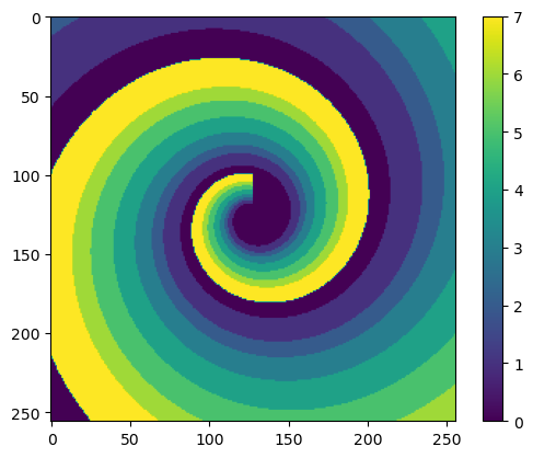
One important thing is to define a point belong to which spiral arm. We can get the spiral arm index with B_generator.indexs.

#visualize the index
indexs = B_generator.indexs.reshape((nx,ny,nz))
plt.imshow(indexs[:,:,32])
plt.colorbar()

<matplotlib.colorbar.Colorbar at 0x7f93fc1c0450>

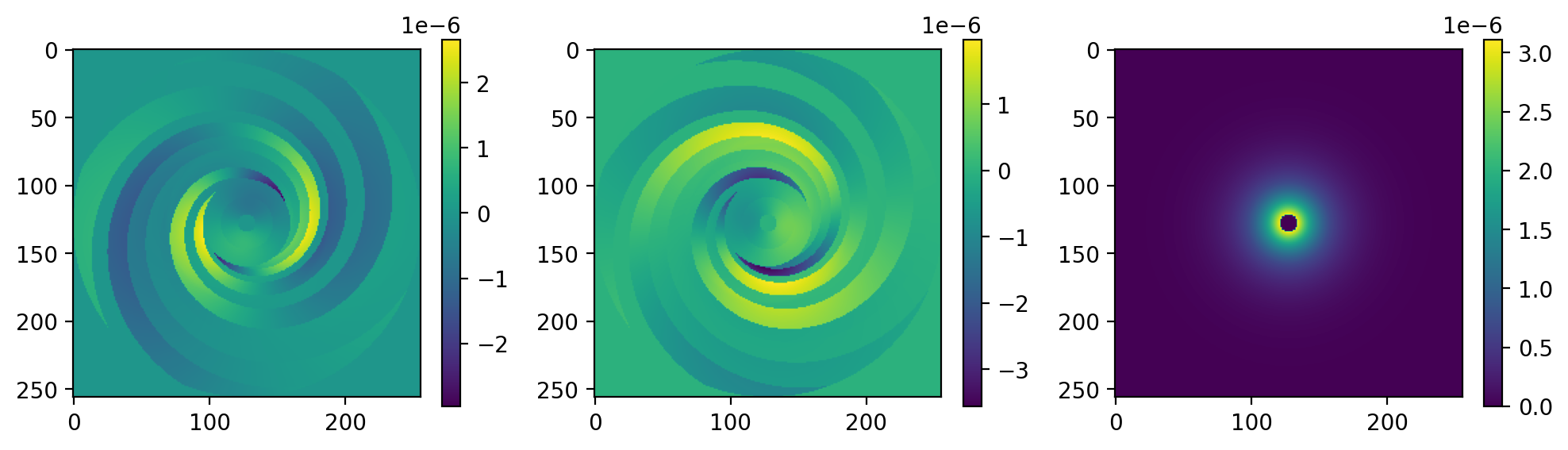
Generate the field. You only need to provide the model parameters

%%time
B_field = B_generator.B_field(jf12_params)#.reshape((nx,ny,nz,3))

CPU times: user 4.8 ms, sys: 3.04 ms, total: 7.84 ms
Wall time: 4.85 ms

plt.figure(dpi=200,figsize=(12,3))

plt.subplot(131)
plt.imshow(B_field[:,:,32,0])
plt.colorbar()

plt.subplot(132)
plt.imshow(B_field[:,:,32,1])
plt.colorbar()

plt.subplot(133)
plt.imshow(B_field[:,:,32,2])
plt.colorbar()

<matplotlib.colorbar.Colorbar at 0x7f93f4154390>

LSA B field

similarly, you can generate the LSA B field on the same grid.

\[\mathbf{B}(r,\phi,z) = b_0[ \cos(\psi(r))\cos(\chi_B(z))\hat{r} +\sin(\psi(r))\cos(\chi_B(z))\hat{\phi}+ \sin(\chi_B(z))\hat{z}]\]

Define the generator

lsa_params = {"b0":1.2,
               "psi0":27.0*np.pi/180,
               "psi1":0.9*np.pi/180,
               "chi0":25.0*np.pi/180}

B_generator = synax.bfield.B_lsa(coords)

Call .B_field() to calculate the field.

%%time
B_field = B_generator.B_field(lsa_params)

CPU times: user 0 ns, sys: 4.08 ms, total: 4.08 ms
Wall time: 2.45 ms

plt.figure(dpi=200,figsize=(12,3))

plt.subplot(131)
plt.imshow(B_field[:,:,32,0])
plt.colorbar()

plt.subplot(132)
plt.imshow(B_field[:,:,32,1])
plt.colorbar()

plt.subplot(133)
plt.imshow(B_field[:,:,32,2])
plt.colorbar()

<matplotlib.colorbar.Colorbar at 0x7f93e42cb050>

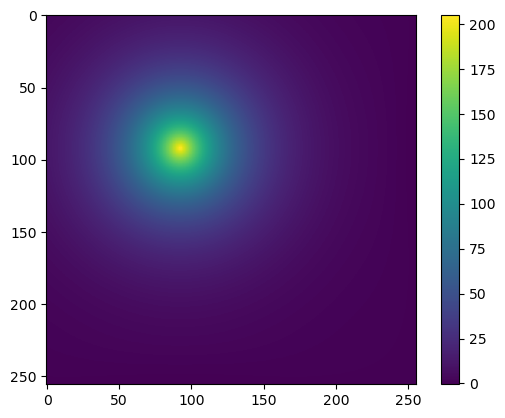
WMAP C field

This is for WMAP C field:

\[C_0(\mathbf{r}) = C_{0}e^{-r/h_r}{\rm sech}^2(z/h_z)\]

C_generator = synax.cfield.C_WMAP(coords)

%%time
WMAP_params = {'C0':211.13068378473076,'hr':5.,'hd':1.}
C_field = C_generator.C_field(WMAP_params)

CPU times: user 1.53 ms, sys: 1.47 ms, total: 3 ms
Wall time: 1.53 ms

plt.imshow(C_field[:,:,32])
plt.colorbar()

<matplotlib.colorbar.Colorbar at 0x7f939406b5d0>

Grid models

All grid field generators are similar. Use thermal electron field generator synax.tefield.TE_grid as a example.

Here we use C_field generated in the previous step as the grid field.

We still need to provide (xs,ys,zs), they are the coordinates along one axis, as regular 3D field can be fully characterized by them.

TE_generator = synax.tefield.TE_grid((coords[0]+5.5,coords[1]+5.5,coords[2]),(xs,ys,zs))

Here the model parameters are exactly field on a 3D grid.

%%time
TE_field = TE_generator.TE_field(C_field)

CPU times: user 8.09 s, sys: 7.25 s, total: 15.3 s
Wall time: 5.78 s

plt.imshow(TE_field[:,:,32])
plt.colorbar()

<matplotlib.colorbar.Colorbar at 0x7f9370644fd0>

coords[2].shape

(256, 256, 64)