Optimizing to reproduce the Haslam map

Here we’ll briefly introduce how to optimize a grid \(\mathbf{B}\) model to produce a Haslam 408 MHz map.

#%env XLA_PYTHON_CLIENT_PREALLOCATE=false
%env XLA_PYTHON_CLIENT_ALLOCATOR=platform

env: XLA_PYTHON_CLIENT_ALLOCATOR=platform

import os
import sys
import jax,blackjax
jax.config.update("jax_enable_x64", True)
#sys.path.append('../synax/')

import synax,importlib
import jax.numpy as jnp
import interpax
import healpy as hp
import numpy as np
import matplotlib.pyplot as plt
from functools import partial
import scipy.constants as const

read observations

Remember replace the filename with your actual directory!

And we will spatial average it to get a NSIDE = 64 map.

from astropy.io import fits

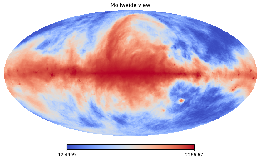
fits_image_filename = '../../SyncEmiss/obs/haslam408_dsds_Remazeilles2014.fits'

data = hp.read_map(fits_image_filename)

data = hp.reorder(data,r2n=True)

data = data.reshape((-1,64)).mean(axis=-1)

data = hp.reorder(data,n2r=True)

hp.mollview(data,norm='hist',cmap='coolwarm')
print(data.shape)

(49152,)

#for debug
def reload_package(package):
    importlib.reload(package)
    for attribute_name in dir(package):
        attribute = getattr(package, attribute_name)
        if type(attribute) == type(package):
            importlib.reload(attribute)

reload_package(synax)

Set up coordinates and fields

During inference, there’re some constant values such as the coordinates, \(n_e\) fields and \(C\) fields. We can pre calculate them to save some time during inference.

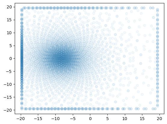
First let’s generate the coordinates.

nside = 64
num_int_points = 512

poss,dls,nhats = synax.coords.get_healpix_positions(nside=nside,num_int_points=num_int_points)
plt.scatter(poss[0,::10,500],poss[1,::10,500],alpha=0.05)
poss.shape

(3, 49152, 512)

Then generate C field

C_generator = synax.cfield.C_WMAP(poss)

C_field = C_generator.C_field()

Then grid \(n_e\) field, read the grids in and construct generator, then interpolate.

nx,ny,nz = 256,256,64

xs,step = jnp.linspace(-20,20,nx,endpoint=False,retstep=True)
xs = xs + step*0.5

ys,step = jnp.linspace(-20,20,ny,endpoint=False,retstep=True)
ys = ys + step*0.5

zs,step = jnp.linspace(-5,5,nz,endpoint=False,retstep=True)
zs = zs + step*0.5

coords = jnp.meshgrid(xs,ys,zs,indexing='ij')
coords[0].shape

(256, 256, 64)

tereg = np.load('te.npy')# read it in.

TE_generator = synax.tefield.TE_grid(poss,(xs,ys,zs))# set up generator
TE_field = TE_generator.TE_field(tereg)# do interpolation

Carry out optimization

Now let’s optimize. The B field generator is also not a variable during inference, we can define one in advance.

First we need to set up coordinate system for this grid \(\mathbf{B}\) field.

Then call synax to get the B_generator

nx,ny,nz = 128,128,32

xs,step = jnp.linspace(-20,20,nx,endpoint=False,retstep=True)
xs = xs + step*0.5

ys,step = jnp.linspace(-20,20,ny,endpoint=False,retstep=True)
ys = ys + step*0.5

zs,step = jnp.linspace(-5,5,nz,endpoint=False,retstep=True)
zs = zs + step*0.5

coords = jnp.meshgrid(xs,ys,zs,indexing='ij')
coords[0].shape

B_generator = synax.bfield.B_grid(poss,(xs,ys,zs))
B_field = jnp.ones((nx,ny,nz,3))*1e-6
B_generator.B_field(B_field).shape

(49152, 512, 3)

set up some constants, including frequency, simer and spectral index.

from datetime import date
rng_key = jax.random.key(42)
simer = synax.synax.Synax(sim_I = True,sim_P=False)
freq = 0.408
spectral_index = 3.

Here our loss function is simply MSE.

@jax.jit
def grid_model(B_field_grid,freq):
    # this function generates the sync I map with a grid B field
    B_field = B_generator.B_field(B_field_grid)

    sync = simer.sim(freq,B_field,C_field,TE_field,nhats,dls,spectral_index)

    return sync['I']


def logdensity_fn(B_field):
    # this function calculates the loss function with a grid B field
    Sync_I = grid_model(B_field,freq)

    return -1*jnp.sum(((Sync_I-data))**2)


B_field = (np.random.randn(nx,ny,nz,3)*1e-6)*jnp.array([1.,1.,0.1])
Sync_I = grid_model(B_field,freq)

hp.mollview(Sync_I,norm='hist',cmap='coolwarm')

logp_grad = jax.value_and_grad(lambda x:-1*logdensity_fn(x))

Now let’s optimize! here we use optax optimizer.

import optax
from tqdm import tqdm

B_field = (np.random.randn(*(nx,ny,nz,3))*1e-6)*jnp.array([1.,1.,0.1])

B_opt = B_field

solver = optax.yogi(learning_rate=1e-6)

opt_state = solver.init(B_opt)# initialize optimizer

loss = []

#create a mask
ones_field = np.ones((nx,ny,nz))

mask = ((coords[0]**2+coords[1]**2)>400)|((coords[0]**2+coords[1]**2)<9)# add a mask to mask inner region and outer region

ones_field[mask] = 1e-10 # can't be 0, 0 would cause polarization angle NaN problem.

mask = jnp.array(ones_field)[:,:,:,jnp.newaxis]

B_opt = B_opt*mask

progress_bar = tqdm(range(200))
for i in progress_bar:
    value,grad = logp_grad(B_opt)
    if jnp.isnan(value):
        break
    loss.append(value)
    updates, opt_state = solver.update(grad, opt_state, B_opt)
    B_opt = optax.apply_updates(B_opt, updates)
    B_opt = B_opt*mask

    info = { 'loss': loss[-1]}

    # Update the postfix with the current info
    progress_bar.set_postfix(info)

100%|██████████| 200/200 [01:11<00:00,  2.79it/s, loss=4319.830813641992]

visualize the results

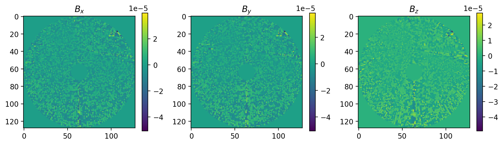
First let’s take a look at the 3 component of the B field at z = 0 kpc.

plt.figure(dpi=200,figsize=(12,3))

plt.subplot(131)
plt.imshow(B_opt[:,:,16,0])
plt.title(r'$B_x$')
plt.colorbar()

plt.subplot(132)
plt.imshow(B_opt[:,:,16,1])
plt.title(r'$B_y$')
plt.colorbar()

plt.subplot(133)
plt.imshow(B_opt[:,:,16,2])
plt.title(r'$B_z$')
plt.colorbar()

<matplotlib.colorbar.Colorbar at 0x7f5768696d50>

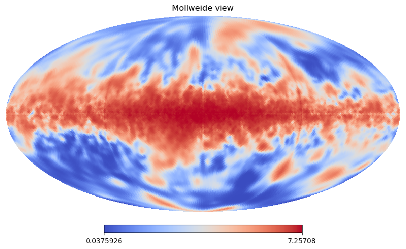
Re-simulate with this optimized \(\mathcal{B}\) field.

Sync_I = grid_model(B_opt,freq)

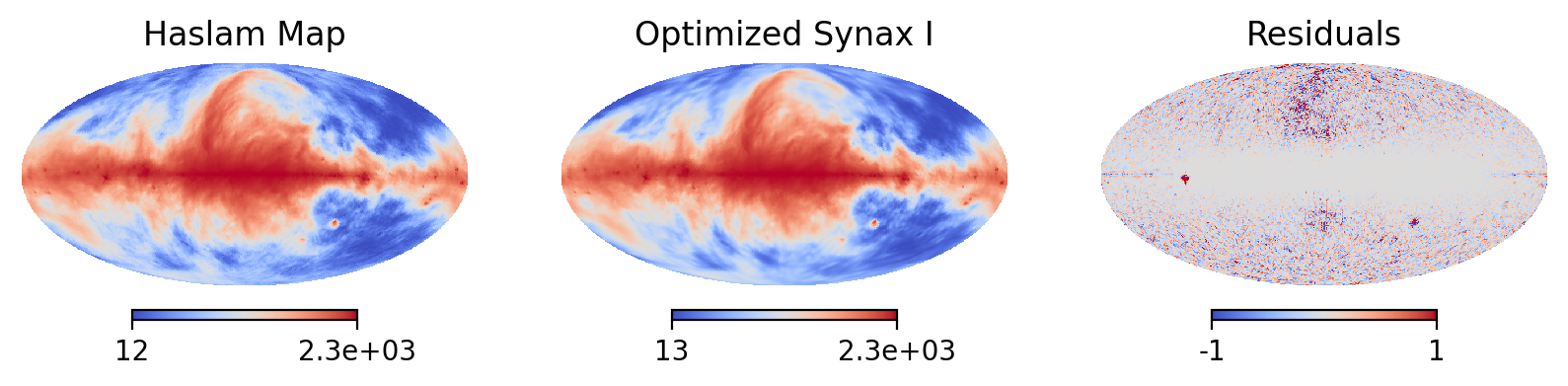
Looks pretty! We did reproduce the Haslam map. However, the degree of freedom is too large to be constrained by a single map. Thus, this optimized B field is not really close to the truth.

But with more constraints we can get a better B field in the future.

plt.figure(dpi=200,figsize=(10,3),)
np.random.seed(42)
plt.subplot(131)
hp.mollview(data,format='%.2g',norm='hist',cmap='coolwarm',hold=True,title='Haslam Map')

plt.subplot(132)
hp.mollview(Sync_I,format='%.2g',norm='hist',cmap='coolwarm',hold=True,title='Optimized Synax I')

plt.subplot(133)
hp.mollview(Sync_I-data,format='%.2g',cmap='coolwarm',hold=True,title='Residuals',max=1,min=-1)


#plt.savefig("../figures/haslam_opt.pdf",bbox_inches='tight',dpi=200)

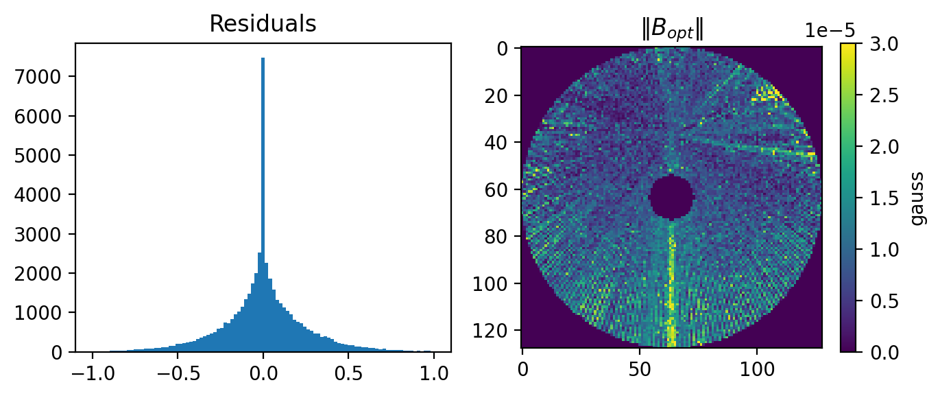
Let’s see the optimized B magnitude. Seems too high, ~10 times of the current estimation.

plt.figure(dpi=200,figsize=(7,3),)

plt.subplot(122)
plt.imshow(((B_opt**2).sum(axis=-1)**(1/2))[:,:,16],vmax=3e-5, vmin=0)
plt.colorbar(label='gauss')
plt.title(r'$\Vert B_{opt} \Vert$')

plt.subplot(121)
plt.hist(Sync_I-data,bins=np.linspace(-1,1,100))
plt.title('Residuals')
plt.tight_layout()
#plt.savefig("../figures/haslam_B.pdf",bbox_inches='tight',dpi=200)

np.std(Sync_I-data)

Array(0.29502564, dtype=float64)